


Updated at: 2022-12-09 03:49:50
Time-series forecast can predict the future by existing historical data. For example, according to the historical access log data of the service, the access request data in the coming week is predicted, and the operators can analyze the problems such as user retention and tap into the essence of the problem according to the prediction results.
A complete time-series forecast task includes two parts: data preview and model computation:
• Data Preview: It is to visualize the data and dimensions that users want to analyze;
• Model Computation: It is to provide a variety of algorithms for users to select different algorithms and parameters for model computation as needed.
To create a new Time -Series Forecast, the specific steps are as follows:
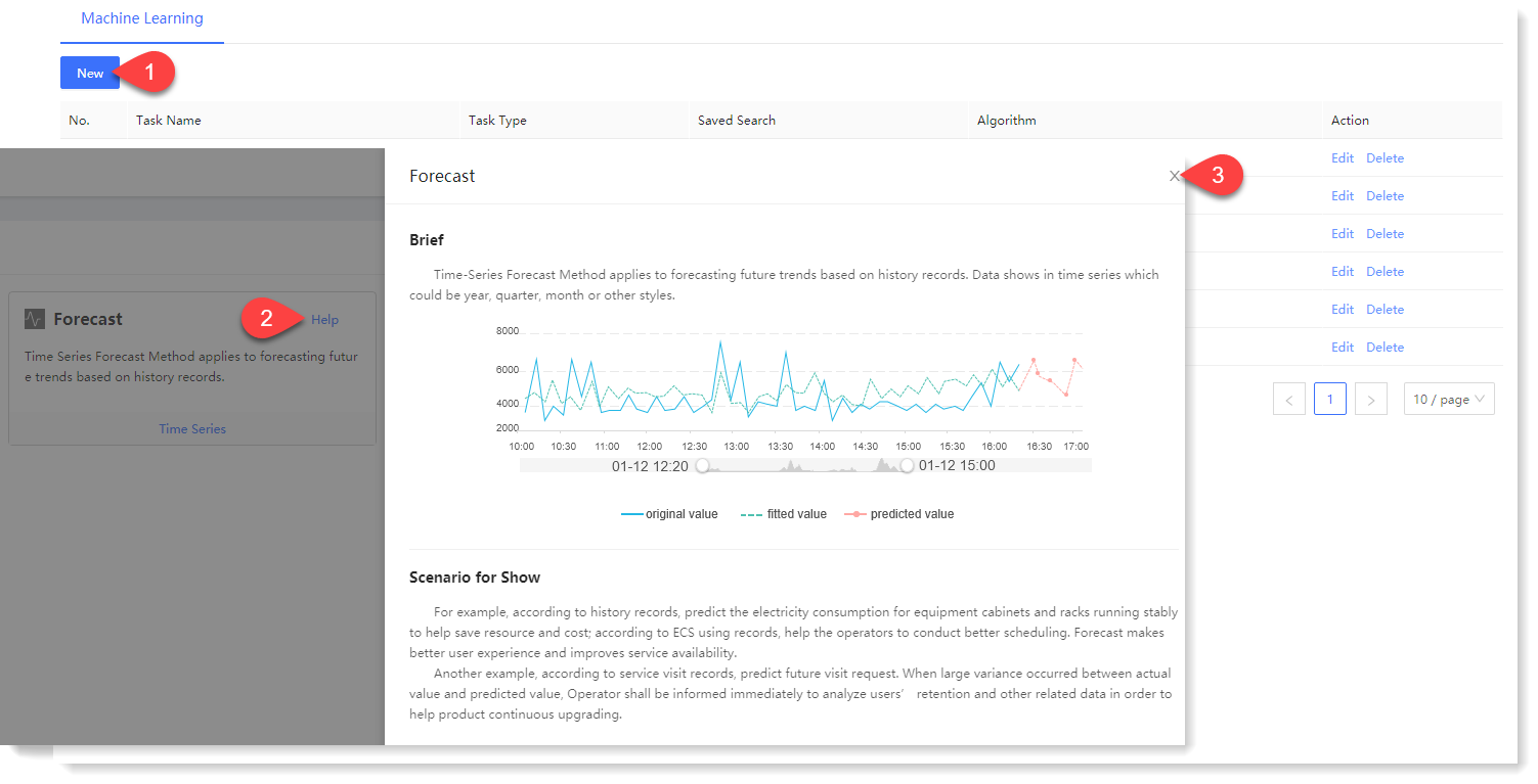
1. Click Machine Learning > New to create New machine learning task, and click Help to view the Brief and Scenario for Show of the time-series detection machine learning task, as follows:
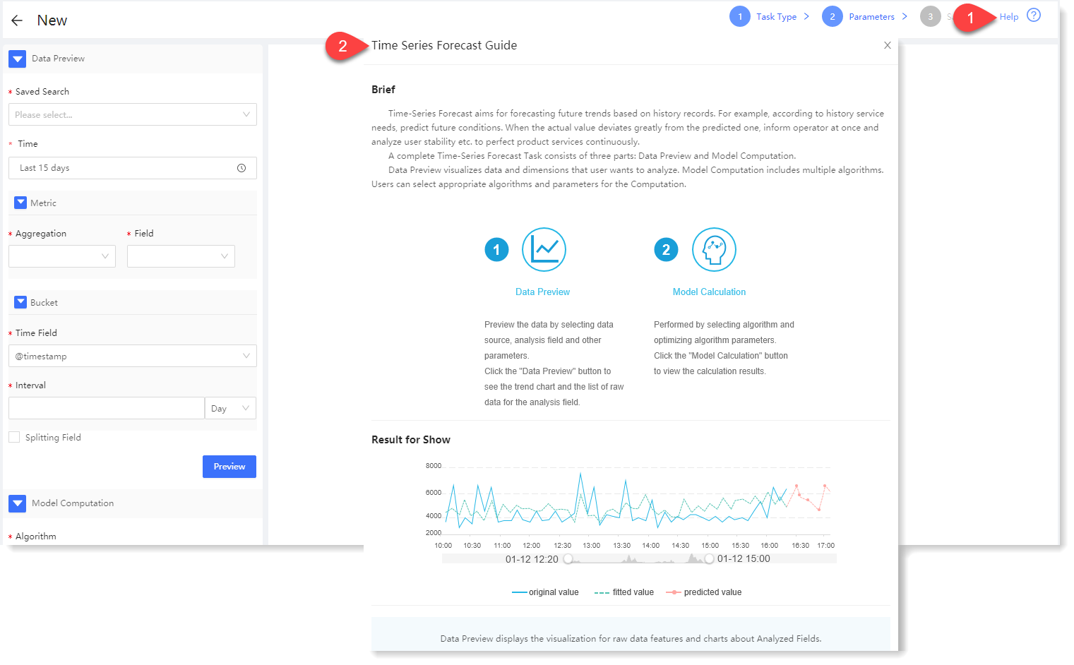
2. Click Time-Series Forecast for parameter configuration, and click Help in the upper right corner to view the brief, usage help, parameter configuration guidance, and algorithm introduction of Time-Series Forecast, as follows:
3. Configuration data preview:
The data preview part is to visualize the original data, data statistics and trend graph.
1) Configure data preview: Fill in the data preview configuration information. During configuring data preview, except that only Time can be selected for Bucket, the rest items are exactly the same. For details, please refer to the section One-Dimensional Anomaly Detection ;
2) Click Preview to view the data preview result, as follows:
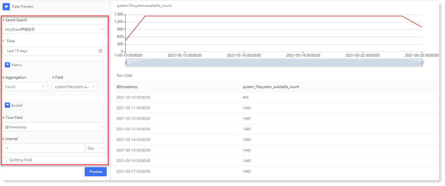
The data preview results include trend graph and Raw Data list: 4. Configure model computation:
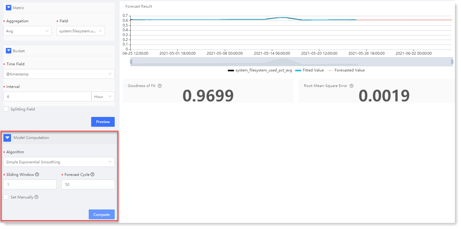
For time-series forecast, three algorithms are currently provided: Simple Exponential Smoothing, Double Exponential Smoothing, and Triple Exponential Smoothing. For some algorithm parameters, AnyRobot can automatically adapt to the parameters. To add manually, you can tick Set Manually for algorithm parameter setting.
• Simple Exponential Smoothing: It is a special weighted average method, suitable for the data of horizontal curves. Click Compute to view the Time-Series Forecast result, as follows:
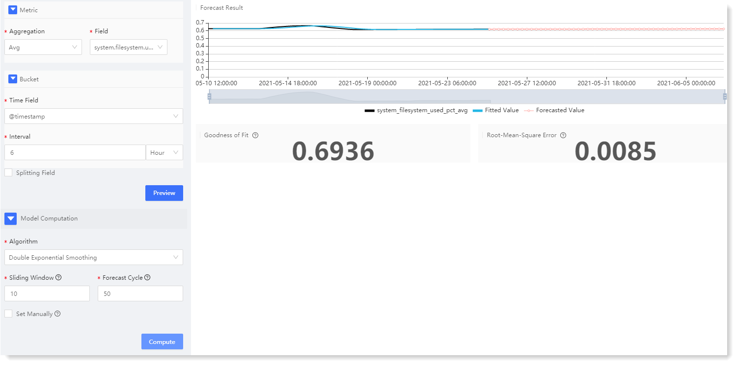
Time-Series Forecast model computation result description: • Double Exponential Smoothing: The smoothing is performed again based on the result of Simple Exponential Smoothing, thus preserving the trend information of data. It is suitable for slope-type time-series data and can predict the time series with trend. Click Compute to view the Time-Series Forecast result, as follows:
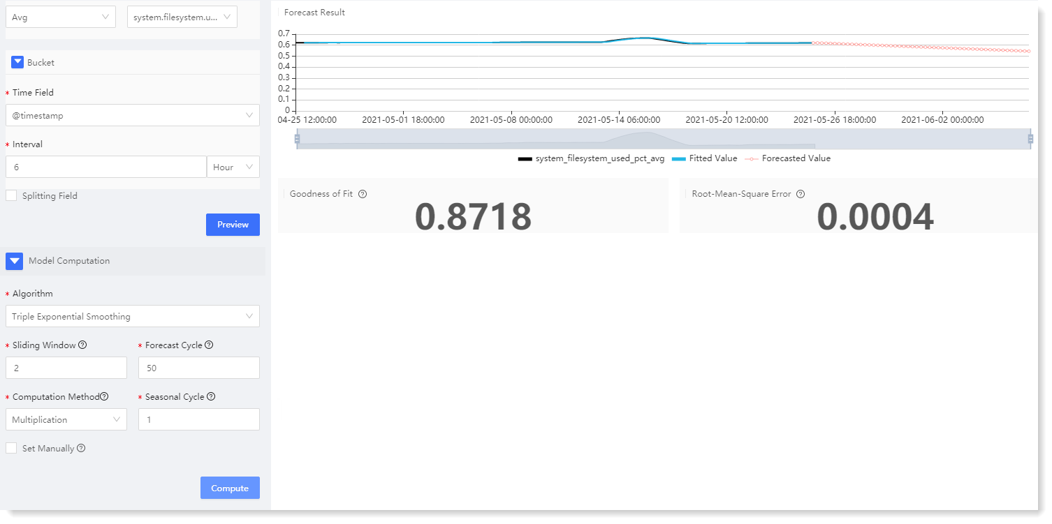
• Triple Exponential Smoothing: Seasonal information is retained on the basis of Double Exponential Smoothing, which can forecast time series with seasonality. It is suitable for trend-type seasonal time series data, and is mostly applied to parabolic data. Click Compute to view the Time-Series Forecast result, as follows:
5. After completing the above configuration, click Save to fill in the machine learning task Name, and click OK to complete the machine learning task creation.
A complete time-series forecast task includes two parts: data preview and model computation:
• Data Preview: It is to visualize the data and dimensions that users want to analyze;
• Model Computation: It is to provide a variety of algorithms for users to select different algorithms and parameters for model computation as needed.
To create a new Time -Series Forecast, the specific steps are as follows:
1. Click Machine Learning > New to create New machine learning task, and click Help to view the Brief and Scenario for Show of the time-series detection machine learning task, as follows:
2. Click Time-Series Forecast for parameter configuration, and click Help in the upper right corner to view the brief, usage help, parameter configuration guidance, and algorithm introduction of Time-Series Forecast, as follows:
3. Configuration data preview:
The data preview part is to visualize the original data, data statistics and trend graph.
1) Configure data preview: Fill in the data preview configuration information. During configuring data preview, except that only Time can be selected for Bucket, the rest items are exactly the same. For details, please refer to the section One-Dimensional Anomaly Detection ;
2) Click Preview to view the data preview result, as follows:
The data preview results include trend graph and Raw Data list: 4. Configure model computation:
For time-series forecast, three algorithms are currently provided: Simple Exponential Smoothing, Double Exponential Smoothing, and Triple Exponential Smoothing. For some algorithm parameters, AnyRobot can automatically adapt to the parameters. To add manually, you can tick Set Manually for algorithm parameter setting.
• Simple Exponential Smoothing: It is a special weighted average method, suitable for the data of horizontal curves. Click Compute to view the Time-Series Forecast result, as follows:
Time-Series Forecast model computation result description: • Double Exponential Smoothing: The smoothing is performed again based on the result of Simple Exponential Smoothing, thus preserving the trend information of data. It is suitable for slope-type time-series data and can predict the time series with trend. Click Compute to view the Time-Series Forecast result, as follows:
• Triple Exponential Smoothing: Seasonal information is retained on the basis of Double Exponential Smoothing, which can forecast time series with seasonality. It is suitable for trend-type seasonal time series data, and is mostly applied to parabolic data. Click Compute to view the Time-Series Forecast result, as follows:
5. After completing the above configuration, click Save to fill in the machine learning task Name, and click OK to complete the machine learning task creation.
< Previous:
Next: >