


Updated at: 2022-12-09 03:49:50
A complete one-dimensional anomaly detection includes 3 parts: data preview, data preprocessing and model computation:
• Data Preview: It is to visualize data analysis dimensions and the result of data analytics;
• Data preprocessing: It is to configure the processing of missing value to avoid the calculation inability due to missing data;
• Model Computation: It is to provide a variety of algorithms for users to select different algorithms and parameters for model computation as needed.
To create a new one-dimensional anomaly detection, the specific steps are as follows:
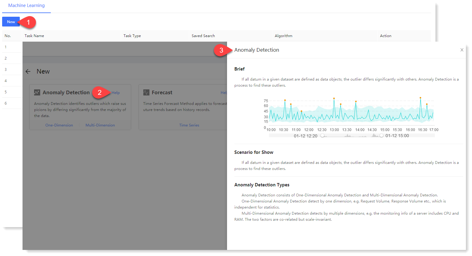
1. Click Machine Learning > New to create New machine learning task, and click Help to view the Brief and Scenario for Show of the anomaly detection machine learning task, as follows:
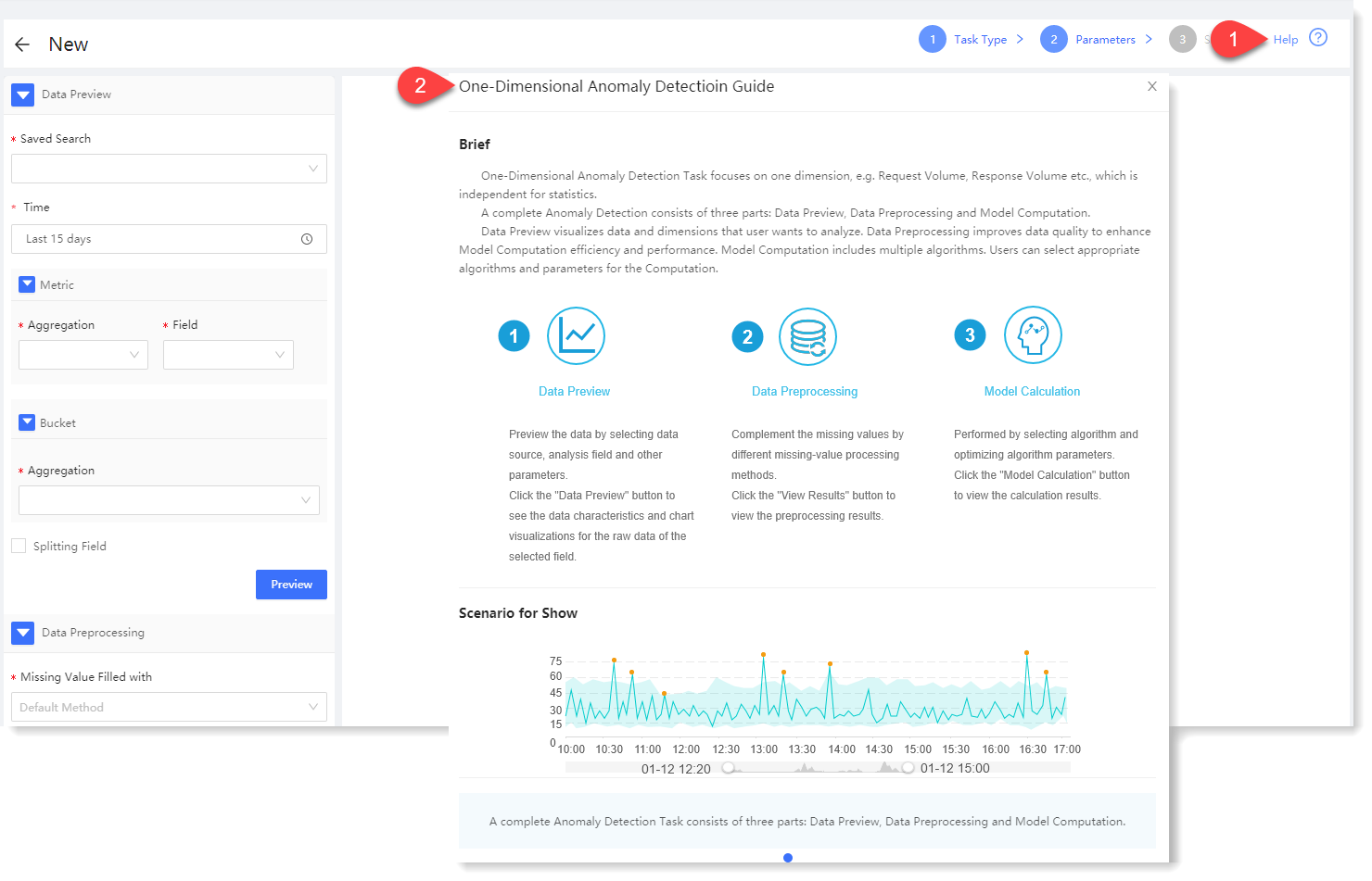
2. Click One-Dimension to make configuration of new one-dimensional anomaly detection parameters. Click Help in the upper right corner to view the brief, usage help, parameter configuration guidance, and algorithm introduction of one-dimensional anomaly detection, as follows:
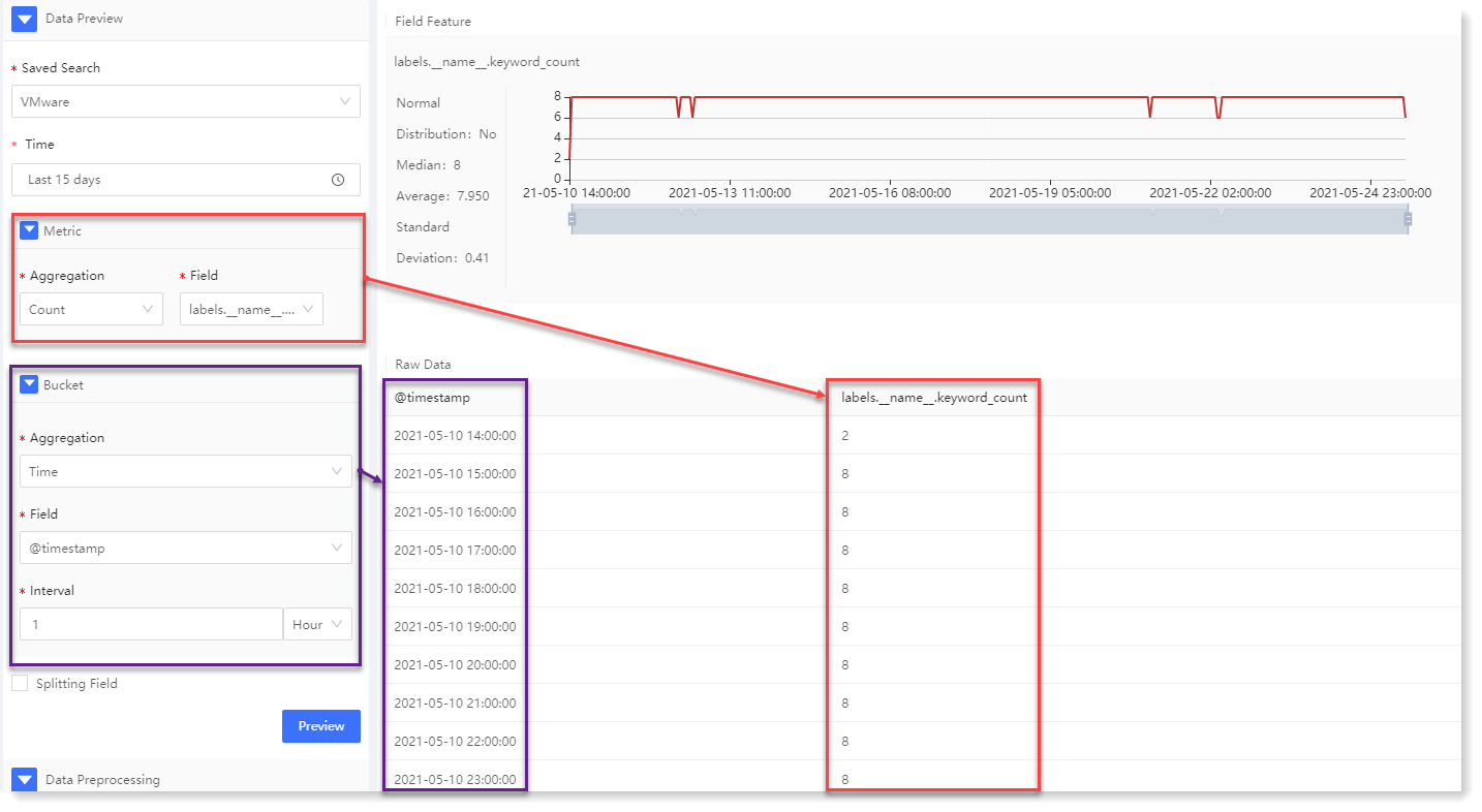
3. Configuration data preview: By configuring the data preview, you can preview the statistical information and trend graph of the data, and view the original data in the preview, as follows:
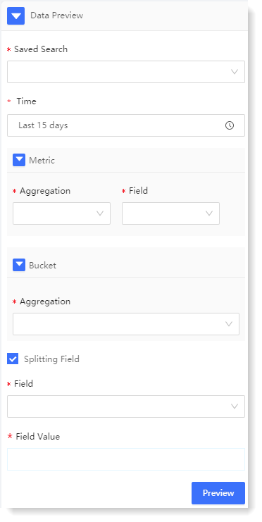
► * Saved Search: In the dropdown list of saved searches, select the required saved searches to filter log data sources.
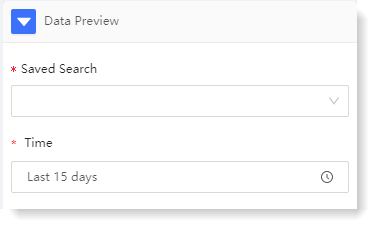
► * Time: It is to filter the selected data by time range, supporting quick selection and time period selection.
► Metric: It includes two parts: Aggregation and Field, indicating the impact dimension to be analyzed. For example: To analyze the number of Apache visits, you can choose count + access users.
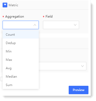
• * Aggregation: It is the aggregation method of the parsing field. It is the aggregation method of the parsing field. It provides Count, Unique Count, Min, Max, Avg, Median, Sum for string type fields, and provide Count and Unique Count for non-string type fields.
• * Field: It is the field to be analyzed.
► Bucket - * Aggregation: The Bucket represents the information on the X axis, and the Aggregation represents the type of the bucket, including two types: Time and Item:
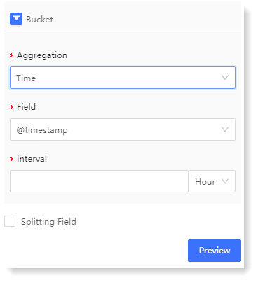
• Time: It means that the X axis is aggregated according to time, and the Time and the Interval need to be selected;
• Item: It means that the X axis is aggregated according to item, and the Item and the Order need to be selected.
► Splitting Field
It indicates whether the selected data needs to be grouped. If Splitting Field is ticked, the data will be grouped according to the Field and Field Value, and each group of data will be calculated separately. If Splitting Field is not ticked, all data will be aggregated, and the preview will display all data results.
• Field: The field that needs to be split, which comes from the field parsed in the selected saved search.
After the parameter configuration, click Preview, the preview result will be displayed on the right side, and the Fields Split List will be displayed after splitting field, as follows:
4. Configuration data preprocessing:
Data preprocessing is to improve data quality for the efficiency and performance of subsequent model computation. The specific configuration is as follows:
1) Configure * Missing Value Filled with: Selecting different missing value processing methods, to make the missing values filled in the data, and improve the quality of the data;
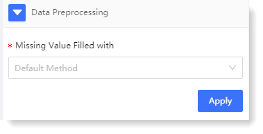
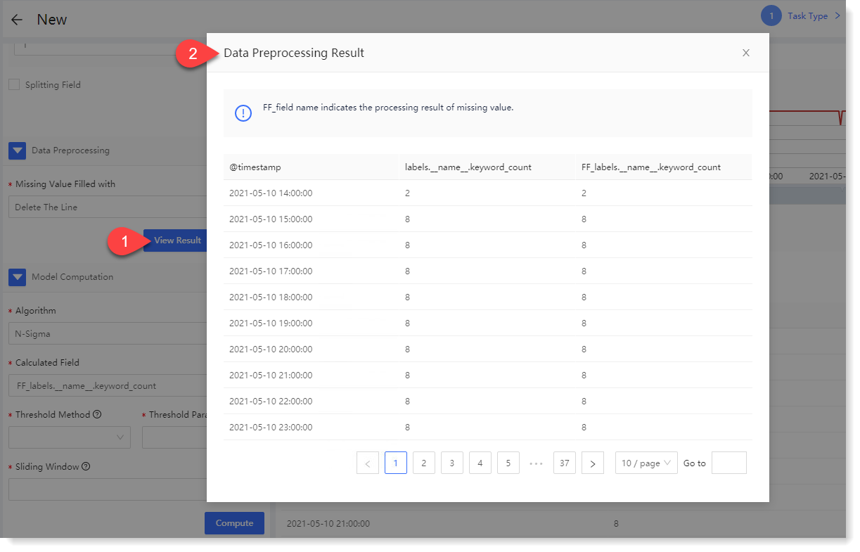
2) Click Apply. After successful execution, you can click View Result to view the field results after data preprocessing, as follows:
5. Configure model computation:
For one-dimensional anomaly detection, currently only N-Sigma algorithm is available. You can calculate the data model through calculated field, threshold calculation method, threshold parameter and configuration in sliding window.
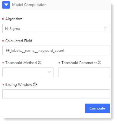
1) The configuration parameters are as follows:
2. Click Compute to view the one-dimensional anomaly detection result, as follows:
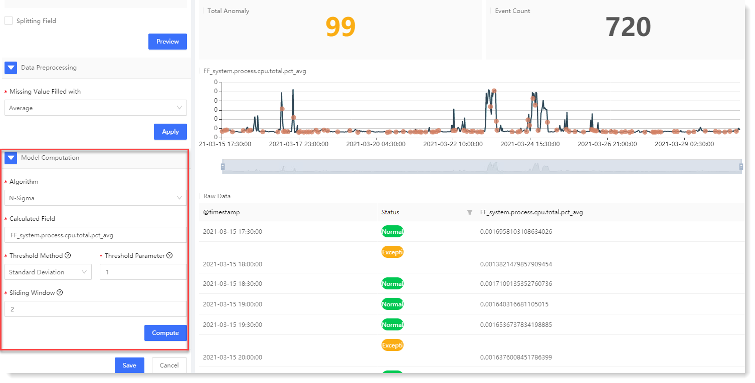
Anomaly detection result description: 6. After completing the above configuration, click Save to fill in the machine learning task Name, and click OK to complete the machine learning task creation.
• Data Preview: It is to visualize data analysis dimensions and the result of data analytics;
• Data preprocessing: It is to configure the processing of missing value to avoid the calculation inability due to missing data;
• Model Computation: It is to provide a variety of algorithms for users to select different algorithms and parameters for model computation as needed.
To create a new one-dimensional anomaly detection, the specific steps are as follows:
1. Click Machine Learning > New to create New machine learning task, and click Help to view the Brief and Scenario for Show of the anomaly detection machine learning task, as follows:
2. Click One-Dimension to make configuration of new one-dimensional anomaly detection parameters. Click Help in the upper right corner to view the brief, usage help, parameter configuration guidance, and algorithm introduction of one-dimensional anomaly detection, as follows:
3. Configuration data preview: By configuring the data preview, you can preview the statistical information and trend graph of the data, and view the original data in the preview, as follows:
► * Saved Search: In the dropdown list of saved searches, select the required saved searches to filter log data sources.
► * Time: It is to filter the selected data by time range, supporting quick selection and time period selection.
► Metric: It includes two parts: Aggregation and Field, indicating the impact dimension to be analyzed. For example: To analyze the number of Apache visits, you can choose count + access users.
• * Aggregation: It is the aggregation method of the parsing field. It is the aggregation method of the parsing field. It provides Count, Unique Count, Min, Max, Avg, Median, Sum for string type fields, and provide Count and Unique Count for non-string type fields.
• * Field: It is the field to be analyzed.
► Bucket - * Aggregation: The Bucket represents the information on the X axis, and the Aggregation represents the type of the bucket, including two types: Time and Item:
• Time: It means that the X axis is aggregated according to time, and the Time and the Interval need to be selected;
• Item: It means that the X axis is aggregated according to item, and the Item and the Order need to be selected.
► Splitting Field
It indicates whether the selected data needs to be grouped. If Splitting Field is ticked, the data will be grouped according to the Field and Field Value, and each group of data will be calculated separately. If Splitting Field is not ticked, all data will be aggregated, and the preview will display all data results.
• Field: The field that needs to be split, which comes from the field parsed in the selected saved search.
• For example: The selected saved search is Apache access log, to be grouped according to each access host, and calculate the user count of each access host;
• Parsing: In the above example, the splitting field is the Host field, the aggregation method of Metric is Count, and the aggregation field of Metric is User.
• Field Value: It is a specific field value to display for the result of Splitting Field. For example: To display 3 hosts from the results of access host, you can select the 3 hosts to be displayed.• Parsing: In the above example, the splitting field is the Host field, the aggregation method of Metric is Count, and the aggregation field of Metric is User.
After the parameter configuration, click Preview, the preview result will be displayed on the right side, and the Fields Split List will be displayed after splitting field, as follows:
4. Configuration data preprocessing:
Data preprocessing is to improve data quality for the efficiency and performance of subsequent model computation. The specific configuration is as follows:
1) Configure * Missing Value Filled with: Selecting different missing value processing methods, to make the missing values filled in the data, and improve the quality of the data;
2) Click Apply. After successful execution, you can click View Result to view the field results after data preprocessing, as follows:
5. Configure model computation:
For one-dimensional anomaly detection, currently only N-Sigma algorithm is available. You can calculate the data model through calculated field, threshold calculation method, threshold parameter and configuration in sliding window.
1) The configuration parameters are as follows:
2. Click Compute to view the one-dimensional anomaly detection result, as follows:
Anomaly detection result description: 6. After completing the above configuration, click Save to fill in the machine learning task Name, and click OK to complete the machine learning task creation.
< Previous:
Next: >