


Updated at: 2022-12-09 03:49:50
Multi-dimensional anomaly detection can be processed and calculated based on data of multiple influence dimensions, and supports Mahalanobis distance model algorithm.
A complete multi-dimensional anomaly detection includes 3 parts: data preview, data preprocessing and model computation:
► Data Preview: It is to visualize the data and dimensions that users want to analyze;
► Data preprocessing: It includes missing value processing and preprocessing configuration:
• Missing value processing configuration: It provides 9 different data missing value processing methods to avoid the calculation inability due to missing data;
• Preprocessing configuration: Preprocessing can be performed according to different methods to improve data quality and the accuracy and performance of subsequent model calculations.
► Model Computation: It is to provide a variety of algorithms for users to select different algorithms and parameters for model computation as needed.
To create a new multi-dimensional anomaly detection, the specific steps are as follows:
1. Click Machine Learning > New to create New machine learning task, and click Help to view the Brief and Scenario for Show of the anomaly detection machine learning task, as follows:
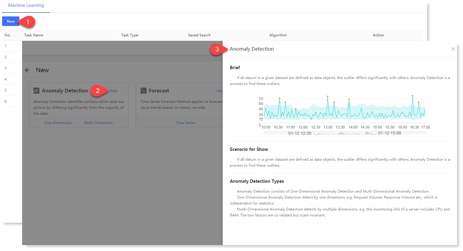
2. Click Multi-Dimension to make configuration of new multi-dimensional anomaly detection parameters. Click Help in the upper right corner to view the brief, usage help, parameter configuration guidance, and algorithm introduction of multi-dimensional anomaly detection, as follows:

3. Configuration data preview:
The data preview part is to visualize the original data, data statistics and trend graph.
1) Configure data preview: Fill in the data preview configuration information. During configuring data preview, except that multiple fields can be added to Metric, the rest are completely the same. For details, please refer to the section One-dimensional Anomaly Detection ;
2) Click Preview to view the data preview result, as follows:
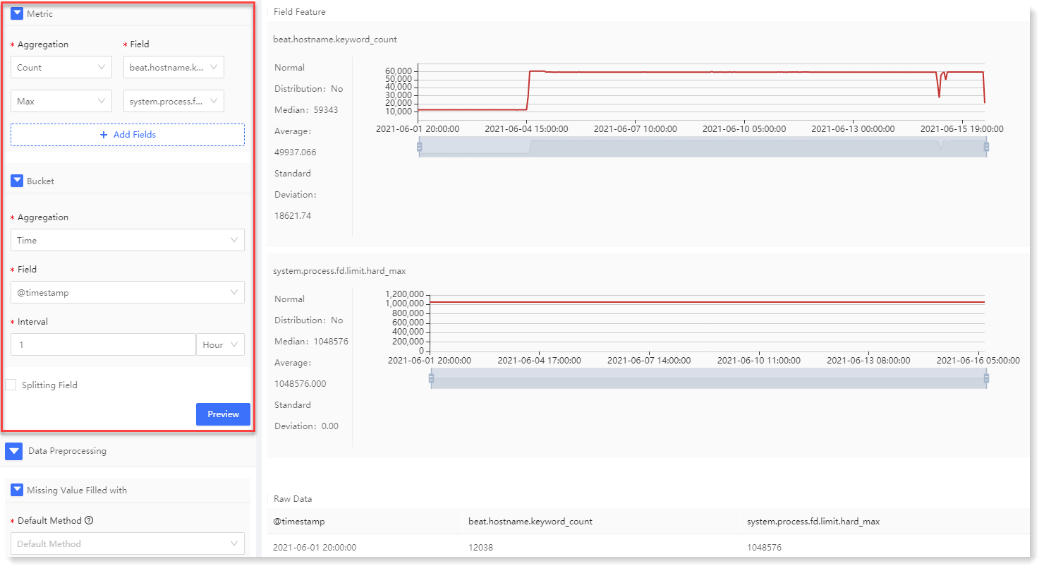
The data preview results include statistics, trend graph and Raw Data list, as follows: 4. Configuration data preprocessing:
Multi-dimensional anomaly detection data preprocessing includes two parts: Missing Value Filled with and Preprocessing.
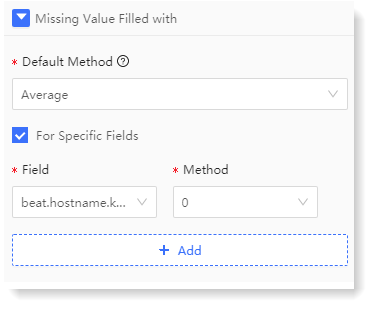
1) Configure Missing Value Filled with: Selecting different missing value processing methods, to make the missing values filled in the data, and improve the quality of the data;
• Configure Default Method: The default method is valid for the selected fields except for specific field;
• To configure the missing value processing method for specific field, you can click Add to set missing value processing for specific field, as follows:
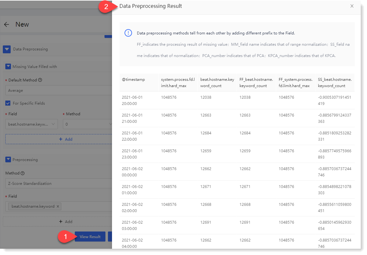
2) Configure Preprocessing: You can choose different methods for data preprocessing. Currently, two methods are available: Standardization and Dimensionality Reduction, and multiple preprocessing tasks can be added;
• Standardization: It is variance calculation, and variance is the comparison of average values. Multi-dimensional anomaly detection supports range standardization and Z-Score standardization;
A complete multi-dimensional anomaly detection includes 3 parts: data preview, data preprocessing and model computation:
► Data Preview: It is to visualize the data and dimensions that users want to analyze;
► Data preprocessing: It includes missing value processing and preprocessing configuration:
• Missing value processing configuration: It provides 9 different data missing value processing methods to avoid the calculation inability due to missing data;
• Preprocessing configuration: Preprocessing can be performed according to different methods to improve data quality and the accuracy and performance of subsequent model calculations.
► Model Computation: It is to provide a variety of algorithms for users to select different algorithms and parameters for model computation as needed.
To create a new multi-dimensional anomaly detection, the specific steps are as follows:
1. Click Machine Learning > New to create New machine learning task, and click Help to view the Brief and Scenario for Show of the anomaly detection machine learning task, as follows:
2. Click Multi-Dimension to make configuration of new multi-dimensional anomaly detection parameters. Click Help in the upper right corner to view the brief, usage help, parameter configuration guidance, and algorithm introduction of multi-dimensional anomaly detection, as follows:
3. Configuration data preview:
The data preview part is to visualize the original data, data statistics and trend graph.
1) Configure data preview: Fill in the data preview configuration information. During configuring data preview, except that multiple fields can be added to Metric, the rest are completely the same. For details, please refer to the section One-dimensional Anomaly Detection ;
2) Click Preview to view the data preview result, as follows:
The data preview results include statistics, trend graph and Raw Data list, as follows: 4. Configuration data preprocessing:
Multi-dimensional anomaly detection data preprocessing includes two parts: Missing Value Filled with and Preprocessing.
1) Configure Missing Value Filled with: Selecting different missing value processing methods, to make the missing values filled in the data, and improve the quality of the data;
• Configure Default Method: The default method is valid for the selected fields except for specific field;
• To configure the missing value processing method for specific field, you can click Add to set missing value processing for specific field, as follows:
2) Configure Preprocessing: You can choose different methods for data preprocessing. Currently, two methods are available: Standardization and Dimensionality Reduction, and multiple preprocessing tasks can be added;
• Standardization: It is variance calculation, and variance is the comparison of average values. Multi-dimensional anomaly detection supports range standardization and Z-Score standardization;
• Range standardization: Range, also known as range error or full range, is used to count the number of outliers in data. Range is the difference between the maximum and minimum values. Range standardization can reflect the fluctuation range of a group of data. The greater the range, the greater the degree of dispersion.
• Z-Score standardization: It is zero-mean standardization, also known as standard deviation standardization, as one of the methods of data standardization processing. It can be used in scenarios where the data distribution is too messy to judge the maximum and minimum values, or there are too many outliers in the data center.
• Z-Score standardization: It is zero-mean standardization, also known as standard deviation standardization, as one of the methods of data standardization processing. It can be used in scenarios where the data distribution is too messy to judge the maximum and minimum values, or there are too many outliers in the data center.
• Dimension reduction: It is a method that can reduce the number of features in a data set while avoiding losing too much information and maintaining or improving model performance, helpful for data visualization. Multidimensional anomaly detection supports PCA and Kernelized PCA:
• PCA (Principal Component Analysis) is a technique for analyzing and simplifying data sets. Its purpose is to compress the dimensions of data and reduce the dimensions (complexity) of source data as much as possible, that is, to extract a new set of variables from a large number of existing variables. However, PCA will lose a small amount of information and can reduce the number of features in regression analysis or clustering analysis;
• Kernelized PCA is based on PCA added with Kernel function to deal with scenario with higher-dimensional data. PCA analysis in higher-dimensional space can be realized through KPCA. For data points that are difficult to be linearly classified in normal linear space, KPCA can be used to find suitable high-dimensional linear classification planes in higher dimensions.
• Kernelized PCA is based on PCA added with Kernel function to deal with scenario with higher-dimensional data. PCA analysis in higher-dimensional space can be realized through KPCA. For data points that are difficult to be linearly classified in normal linear space, KPCA can be used to find suitable high-dimensional linear classification planes in higher dimensions.
3) Click Apply. After successful execution, you can click View Result to view the field results after data preprocessing, as follows:
5. Configure model computation:
Multi-dimensional anomaly detection supports Mahalanobis Distance algorithm. You can calculate the data model through calculated field, threshold calculation method, threshold parameter and configuration in sliding window.
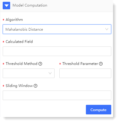
1) The configuration parameters are as follows: 2) Click Compute to view the multi-dimensional anomaly detection result, as follows:
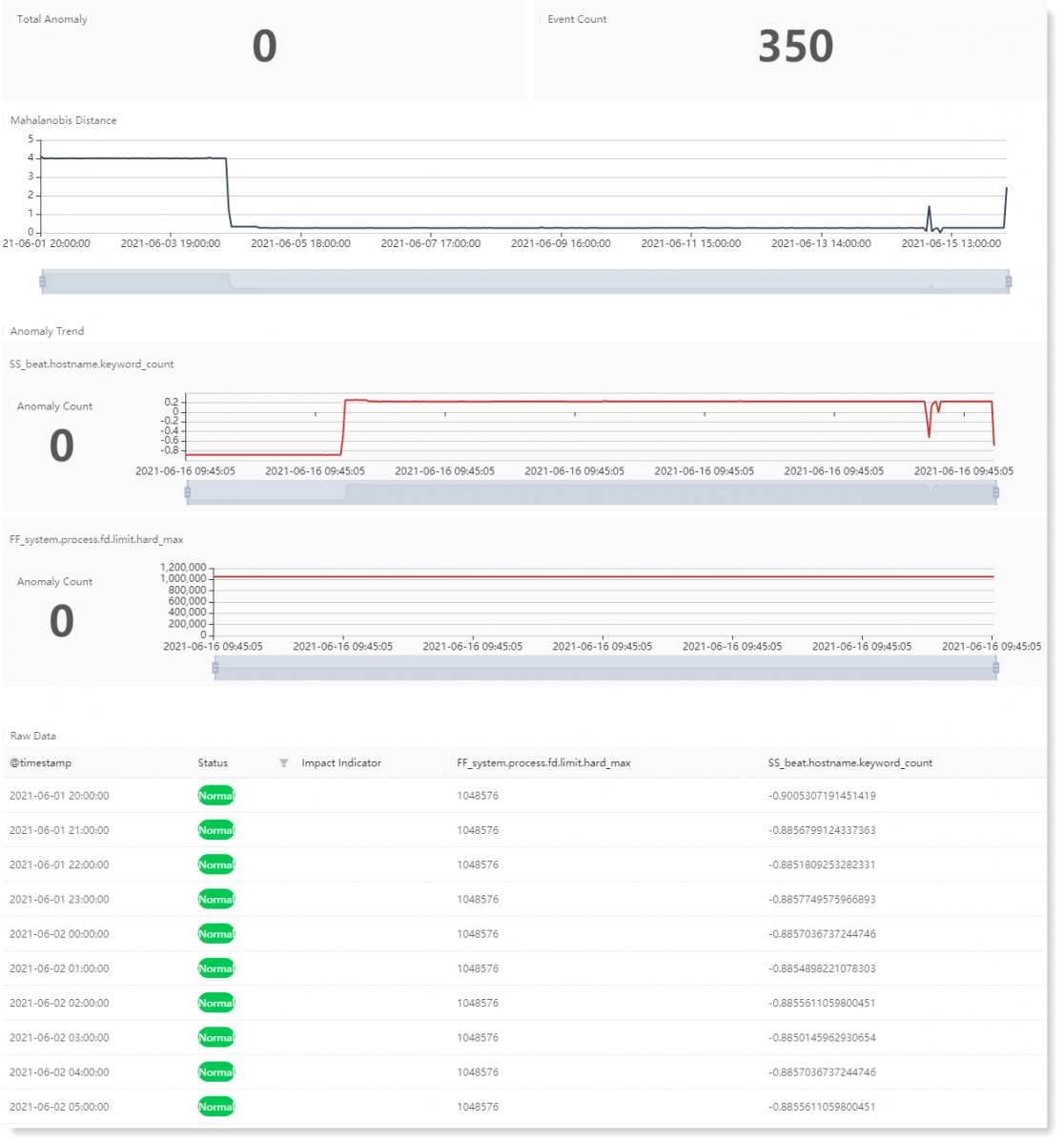
Multi-dimensional anomaly detection model computation result description:
6. After completing the above configuration, click Save to fill in the machine learning task Name, and click OK to complete the machine learning task creation.5. Configure model computation:
Multi-dimensional anomaly detection supports Mahalanobis Distance algorithm. You can calculate the data model through calculated field, threshold calculation method, threshold parameter and configuration in sliding window.
1) The configuration parameters are as follows: 2) Click Compute to view the multi-dimensional anomaly detection result, as follows:
< Previous:
Next: >